Chapter 4 Learning behaviours

In this chapter, we present the first contribution, which is the learning part from the conceptual architecture presented in Figure 3.2. Section 4.1 begins with an overview of this contribution, recalls the research question, explains its motivations, and presents a schema derived from the conceptual architecture, focusing on the learning part, and showing its internal mechanisms. Sections 4.2 and 4.3 presents the components necessary to our algorithms, and algorithms are then described in Section 4.4. We detail the experiment setup, based on the multi-agent Smart Grid use-case presented in Section 3.4, in Section 4.5, and Section 4.6 reports the results. A discussion of these algorithms’ advantages and drawbacks is finally presented in Section 4.7.

4.1 Overview

We recall that the aim of this first contribution is to answer the first research question: How to learn behaviours aligned with moral values, using Reinforcement Learning with complex, continuous, and multi-dimensional representations of actions and situations? How to make the multiple learning agents able to adapt their behaviours to changes in the environment?

To do so, we propose 2 Reinforcement Learning algorithms. These algorithms needed to have 2 important properties: 1) to be able to handle multi-dimensional domains, for both states and actions, as per our hypothesis H2, and as motivated in our state of the art of Machine Ethics. 2) to be a modular approach, as per the “incremental approach” principle of our methodology. Indeed, the algorithms were meant as a first step, a building basis on top of which we would add improvements and features throughout our next contributions. In order to facilitate these improvements, modularity was important, rather than implementing an end-to-end architecture, as is often found in Deep Neural Networks. Such networks, while achieving impressive performance on their tasks, can be difficult to reuse and modify. As we will see in the results, our algorithms obtain similar or even better performance.

The algorithms that we propose are based on an existing work (Smith, 2002a, 2002b) that we extend and evaluate in a more complex use-case. Smith’s initial work proposed, in order to handle continuous domains, to associate Self-Organizing Maps (SOMs) to a Q-Table. This idea fulfills the first property, and also offers the modularity required by the second: by combining elements, it allows to easily modify, replace, or even add one or several elements to the approach. This motivated our choice of extending Smith’s work.

First, we explain what is a Q-Table from the Q-Learning algorithm, and its limitations. We then present Self-Organizing Maps, the Dynamic Self-Organizing Map variation, and how we can use them to solve the Q-Table’s limitations. We combine these components to propose an extension of Smith’s algorithm that we name Q-SOM, which leverages a Q-Table and Self-Organizing Maps (SOMs), and a new algorithm named Q-DSOM, which leverages a Q-Table and Dynamic SOMs (DSOMs).

Learning agents presented in this chapter correspond to prosumer agents in Figure 3.4. They receive observations and take actions; during our experiments, these observations and actions are those described in this figure and more generally in Section 3.4.

Figure 4.1 presents a summarizing schema of our proposed algorithms. It includes multiple learning agents that live within a shared environment. This environment sends observations to agents, which represent the current state, so that agents may choose an action and perform it in the environment. In response, the environment changes its state, and sends them new observations, potentially different for each agent, corresponding to this new state, as well as a reward indicating how correct the performed action was. Learning agents leverage the new observations and the reward to update their internal model. This observation-action-reward cycle is then repeated so as to make learning agents improve their behaviour, with respect to the considerations embedded in the reward function. The decision process relies on 3 structures, a State (Dynamic) Self-Organizing Map, also named the State-(D)SOM, an Action (Dynamic) Self-Organizing Map, also named the Action-(D)SOM, and a Q-Table. They take observations as inputs and output an action, which are both vectors of continuous numbers. The learning process updates these same structures, and takes the reward as an input, in addition to observations.

Figure 4.1: Architecture of the Q-SOM and Q-DSOM algorithms, which consist of a decision and learning processes. The processes rely on a State-(D)SOM, an Action-(D)SOM, and a Q-Table.

4.2 Q-Table

The Q-Table is the central component of the well-known Q-Learning algorithm (Watkins & Dayan, 1992). It is tasked with learning the interest of a state-action pair, i.e., the expected horizon of received rewards for taking an action in a given state. As we saw in Section 2.2, the Q-Table is a tabular structure, where rows correspond to possible states, and columns to possible actions, such that the row $\Q(s, \cdot)$ gives the interests of taking every possible action in state $s$, and, more specifically, the cell $\Q(s, a)$ is the interest of taking action $a$ in state $s$. These cells, also named Q-Values, can be learned iteratively by collecting experiences of interactions, and by applying the Bellman equation.

We recall that the interests take into account both the short-term immediate reward, but also the interest of the following state $s'$, resulting from the application of $a$ in $s$. Thus, an action that leads to a state where any action yields a low reward, or in other word an unattractive state, would have a low interest, regardless of its immediate reward.

Assuming that the Q-Values have converged towards the “true” interests, the optimal policy can be easily obtained through the Q-Table, by selecting the action with the maximum interest in each state. By definition, this “best action” will lead to states with high interests as well, thus yielding, in the long-term, the maximum expected horizon of rewards.

An additional advantage of the Q-Table is the ability to directly have access to the interests, in comparison to other approaches, such as Policy Gradient, which typically manipulate actions’ probabilities, increasing and decreasing them based on received rewards. These interests can be conveyed to humans to support or detail the algorithm’s decision process, an advantage that we will exploit later, in Chapter 6.

Nevertheless, Q-Tables have an intrinsic limitation: they are defined as a tabular structure. This structure works flawlessly in simple environments, e.g., those with a few discrete states and actions. Yet, in more complex environments, especially those that require continuous representations of states and actions, it is not sufficient any more, as we would require an infinite number of rows and columns, and therefore an infinite amount of memory. Additionally, because of the continuous domains’ nature, it would be almost impossible to obtain twice the exact same state: the cells, or Q-Values, would almost always get at most a single interaction, which does not allow for adequate learning and convergence towards the true interests.

To counter this disadvantage, we rely on the use of Self-Organizing Maps (SOMs) that handle the continuous domains. The mechanisms of SOMs are explained in the next section, and we detail how they are used in conjunction with a Q-Table in Section 4.4.

4.3 (Dynamic) Self-Organizing Maps

A Self-Organizing Map (SOM) (Kohonen, 1990) is an artificial neural network that can be used for unsupervised learning of representations for high-dimensional data. SOMs contain a fixed set of neurons, typically arranged in a rectangular 2D grid, which are associated to a unique identifier, e.g., neuron #1, neuron #2, etc., and a vector, named the prototype vector. Prototype vectors lie in the latent space, which is the highly dimensional space the SOM must learn to represent.

The goal is to learn to represent as closely as possible the distribution of data within the latent space, based on the input data set. To do so, prototype vectors are incrementally updated and “moved” towards the different regions of the latent space that contain the most data points. Each time an input vector, or data point, is presented to the map, the neurons compete for attention: the one with the closest prototype vector to the input vector is named the Best Matching Unit (BMU). Neurons’ prototypes are then updated, based on their distance to the BMU and the input vector. By doing this, the neurons that are the closest to the input vector are moved towards it, whereas the farthest neurons receive little to no modification, and thus can focus on representing different parts of the latent space.

As the number of presented data points increases, the distortion, i.e., the distance between each data point and its closest prototype, diminishes. In other words, neurons’ prototypes are increasingly closer to the real (unknown) distribution of data.

When the map is sufficiently learned, it can be used to perform a mapping of high dimensional data points into a space of lower dimension. Each neuron represents the data points that are closest to its prototype vector. Conversely, each data point is represented by the neuron whose prototype is the closest to its own vector.

This property of SOMs allows us to handle continuous, and multi-dimensional state and action spaces.

Figure 4.2 summarizes and illustrates the training of a SOM. The blue shape represents the data distribution that we wish to learn, from a 2D space for easier visualization. Typically, data would live in higher dimension spaces. Within the data distribution, a white disc shows the data point that is presented to the SOM at the current iteration step. SOM neurons, represented by black nodes, and connected to their neighbors by black edges, are updated towards the current data point. Among them, the Best Matching Unit, identified by an opaque yellow disc, is the closest to the current data point, and as such receives the most important update. The closest neighbors of the BMU, belonging to the larger yellow transparent disc, are also slightly updated. Farther neurons are almost not updated. The learned SOM is represented on the right side of the figure, in which neurons correctly cover the data distribution.

Figure 4.2: Training of a SOM, illustrated on several steps. Image extracted from Wikipedia.

The update received by a neuron is determined by Equation (4.1), with $v$ being the index of the neuron, $\mathbf{W_v}$ is the prototype vector of neuron $v$, $\mathbf{D_t}$ is the data point presented to the SOM at step $t$. $u$ is the index of the Best Matching Unit, i.e., the neuron that satisfies $u = \argmin_{\forall v} \left\|\mathbf{D_t} - \mathbf{W_v}\right\|$.

$$\begin{equation} \mathbf{W_{v}^{t+1}} \gets \mathbf{W_{v}^{t}} + \theta(u, v, t) \alpha(t) \left(\mathbf{D_t} - \mathbf{W_{v}^{t}}\right) \tag{4.1} \end{equation}$$

In this equation, $\theta$ is the neighborhood function, which is typically a gaussian centered on the BMU ($u$), such that the BMU is the most updated, its closest neighbors are slightly updated, and farther neurons are not updated. The learning rate $\alpha$, and the neighborhood function $\theta$ both depend on the time step $t$: they are often monotonically decreasing, in order to force neurons’ convergence and stability.

One of the numerous extensions of the Self-Organizing Map is the Dynamic Self-Organizing Map (DSOM) (Rougier & Boniface, 2011). The idea behind DSOMs is that self-organization should offer both stability, when the input data does not change much, and dynamism, when there is a sudden change. This stems from neurological inspiration, since the human brain is able to both stabilize after the early years of development, and dynamically re-organize itself and adapt when lesions occur.

As we mentioned, the SOM enforces stability through decreasing parameters (learning rate and neighborhood), however this also prevents dynamism. Indeed, as the parameters approach $0$, the vectors’ updates become negligible, and the system does not adapt any more, even when faced with an abrupt change in the data distribution.

DSOMs propose to replace the time-dependent parameters by a time-invariant one, named the elasticity, which determines the coupling of neurons. Whereas SOMs and other similar algorithms try to learn the density of data, DSOMs focus on the structure of the data space, and the map will not try to place several neurons in a high-density region. In other words, if a neuron is considered as sufficiently close to the input data point, the DSOM will not update the other neurons, assuming that this region of the latent space is already quite well represented by this neuron. The “sufficiently close” is determined through the elasticity parameter: with high elasticity, neurons are tightly coupled with each other, whereas lower elasticity let neurons spread out over the whole latent space.

DSOMs replace the update equation with the following:

$$\begin{equation} \mathbf{W_i^{t+1}} \leftarrow \alpha\left\|\mathbf{D_t} - \mathbf{W_i^t}\right\|h_{\eta}(i, u, \mathbf{D_t})\left(\mathbf{D_t} - \mathbf{W_i^t}\right) \tag{4.2} \end{equation}$$

$$\begin{equation} h_{\eta}(i, u, \mathbf{D_t}) = \exp\left( - \frac{1}{\eta^{2}} \frac{\left\| \pos(i) - \pos(u) \right\|^{2}}{\left\| \mathbf{D_t} - \mathbf{W_u} \right\|^{2}} \right) \tag{4.3} \end{equation}$$

where $\alpha$ is the learning rate, $i$ is the index of the currently updated neuron, $\mathbf{D_t}$ is the current data point, $u$ is the index of the best matching unit, $\eta$ is the elasticity parameter, $h_{\eta}$ is the neighborhood function, and $\pos(i)$, $\pos(u)$ are respectively the positions of neurons $i$ and $u$ in the grid (not in the latent space). Intuitively, the distance between $\pos(i)$ and $\pos(u)$ is the minimal number of consecutive neighbors that form a path between $i$ and $u$.

4.4 The Q-SOM and Q-DSOM algorithms

We take inspiration from Decentralized Partially-Observable Markovian Decision Processes (DecPOMDPs) to formally describe our proposed algorithms. DecPOMDPs are an extension of the well-known Markovian Decision Process (MDP) that considers multiple agents taking repeated decisions in multiple states of an environment, by receiving only partial observations about the current state. In contrast with the original DecPOMDP as described by Bernstein (Bernstein, Givan, Immerman, & Zilberstein, 2002), we explicitly define the set of learning agents, and we assume that agents receive (different) individual rewards, instead of a team reward.

Definition 4.1 (DecPOMDP) A Decentralized Partially-Observable Markovian Decision Process is a tuple $\left\langle \LAgts, \StateSpace, \ActionSpace, \texttt{T}, \ObsSpace, \texttt{O}, \RewardFn, \gamma \right\rangle$, where:

• $\LAgts$ is the set of learning agents, of size $n = \length{\LAgts}$.
• $\StateSpace$ is the state space, i.e., the set of states that the environment can possibly be in. States are not directly accessible to learning agents.
• $\ActionSpace_l$ is the set of actions accessible to agent $l$, $\forall l \in \LAgts$ as all agents take individual actions. We consider multi-dimensional and continuous actions, thus we have $\ActionSpace_{l} \subseteq \RR^d$, with $d$ the number of dimensions, which depends on the case of application.
• $\ActionSpace$ is the action space, i.e., the set of joint-actions that can be taken at each time step. A joint-action is the combination of all agents’ actions, i.e., $\ActionSpace = \ActionSpace_{l_1} \times \cdots \times \ActionSpace_{l_n}$.
• $\texttt{T}$ is the transition function, defined as $\texttt{T} : \StateSpace \times \ActionSpace \times \StateSpace \rightarrow [0,1]$. In other words, $\texttt{T}(s' | s, \mathbf{a})$ is the probability of obtaining state $\mathbf{s}'$ after taking the action $\mathbf{a}$ in state $\mathbf{s}$.
• $\ObsSpace$ is the observation space, i.e., the set of possible observations that agents can receive. An observation is a partial information about the current state. Similarly to actions, we define $\ObsSpace_{l}$ as the observation space for learning agent $l$, $\forall l \in \LAgts$. As well as actions, observations are multi-dimensional and continuous, thus we have $\ObsSpace_{l} \subseteq \RR^{g}$, with $g$ the number of dimensions, which depends on the use case.
• $\texttt{O}$ is the observation probability function, defined as $\texttt{O} : \ObsSpace \times \StateSpace \times \ActionSpace \rightarrow [0,1]$, i.e., $\texttt{O}(\mathbf{o} | s', \mathbf{a})$ is the probability of receiving the observations $\mathbf{o}$ after taking the action $\mathbf{a}$ and arriving in state $s'$.
• $\RewardFn$ is the reward function, defined as $\forall l \in \LAgts \quad \RewardFn_{l} : \StateSpace \times \ActionSpace_l \rightarrow \RR$. Typically, the reward function itself will be the same for all agents, however, agents are rewarded individually, based on their own contribution to the environment through their action. In other words, $\RewardFn_{l}(s, \mathbf{a}_{l})$ is the reward that learning agent $l$ receives for taking action $\mathbf{a}_{l}$ in state $s$.
• $\gamma$ is the discount factor, to allow for potentially infinite horizon of time steps, with $\gamma \in [0,1[$.

The RL algorithm must learn a stochastic strategy $\pi_{l}$, defined as $\pi_{l} : \ObsSpace_{l} \times \ActionSpace_{l} \rightarrow [0,1]$. In other words, given the observations $\mathbf{o}_{l}$ received by an agent $l$, $\pi(\mathbf{o}_{l}, \mathbf{a})$ is the probability that agent $l$ will take action $\mathbf{a}$.

We recall that observations and actions are vectors of floating numbers, the RL algorithm must therefore handle this accordingly. However, it was mentioned in Section 4.2 that the Q-Table is not suitable for continuous data. To solve this, we take inspiration from an existing work (Smith, 2002a, 2002b) and propose to use variants of Self-Organizing Maps (SOMs) (Kohonen, 1990).

We can leverage SOMs to learn to handle the observation and action spaces: neurons learn the topology of the latent space and create a discretization. By associating each neuron with a unique index, we are able to discretize the multi-dimensional data: each data point is recognized by the neuron with the closest prototype vector, and thus is represented by a discrete identifier, i.e., the neuron’s index.

The proposed algorithms are thus based on 2 (Dynamic) SOMs, a State-SOM, and an Action-SOM, which are associated to a Q-Table. To navigate the Q-Table and access the Q-Values, we use discrete identifiers obtained from the SOMs. The Q-Table’s dimensions thus depend on the (D)SOMs’ number of neurons: the Q-Table has exactly as many rows as the State-(D)SOM has neurons, and exactly as many columns as the Action-(D)SOM has neurons, such that each neuron is represented by a row or column, and reciprocally.

Our algorithms are separated into 2 distinct parts: the decision process, which chooses an action from received observations about the environment, and the learning process, which updates the algorithms’ data structures, so that the next decision step will yield a better action. We present in details these 2 parts below.

4.4.1 The decision process

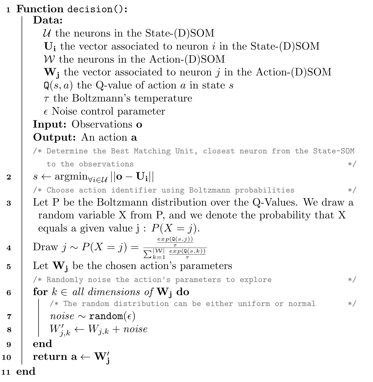
Figure 4.3: Decision algorithm

Figure 4.4: Dataflow of the Q-(D)SOM decision process.

We now explain the decision process that allows an agent to choose an action from received observations, which is described formally in Algorithm 4.3 and represented in Figure 4.4. First, we need to obtain a discrete identifier from an observation $\mathbf{o}$ that is a vector $\in \ObsSpace_l \subseteq \RR^{g}$, in order to access the Q-Table. To do so, we look for the Best Matching Unit (BMU), i.e., the neuron whose prototype vector is the closest to the observations, from the State-SOM, which is the SOM tasked with learning the observation space. The unique index of the BMU is used as the state identifier $s$ (line 2).

We call this identifier a “state hypothesis”, and we use it to navigate the Q-Table and obtain the expected interest of each action, assuming we have correctly identified the state. Knowing these interests $\Q(s,.)$ for all actions, we can assign a probability of taking each one, using a Boltzmann distribution (line 3). Boltzmann is a well-known and used method in RL that helps with the exploration-exploitation dilemma. Indeed, as we saw in Section 2.2, agents should try to maximize their expectancy of received rewards, which means they should exploit high-rewarding actions, i.e., those with a high interest. However, the true interest of the action is not known to agents: they have to discover it incrementally by trying actions into the environment, in various situations, and memorizing the associated reward. If they only choose the action with the maximum interest, they risk focusing on few actions, thus not exploring the others. By not sufficiently exploring, they maintain the phenomenon, as not explored actions will stay at a low interest, reducing their probability of being chosen, and so on. Using Boltzmann mitigates this problem, by giving similar probabilities to similar interests, and yet, a non-zero probability of being chosen even for actions with low interests.

The Boltzmann probability of an action $j$ being selected is computed based on the action’s interest, in the current state, relatively to all other actions’ interests, as follows:

$$\begin{equation} P(X = j) = \frac{ \frac{\exp(\Q(s,j))}{\tau} }{\sum_{k = 1}^{\length{\mathcal{W}}} \frac{\exp(\Q(s,k))}{\tau}} \tag{4.4} \end{equation}$$

Traditionally, the Boltzmann parameter $\tau$ should be decreasing over the time steps, such that the probabilities of high-interest actions will rise, whereas low-interest actions will converge towards a probability of $0$. This mechanism ensures the convergence of the agents’ policy towards the optimal one, by reducing exploration in later steps, in favour of exploitation. However, and as we have already mentioned, we chose to disable the convergence mechanisms in our algorithms, because it prevents, by principle, continuous learning and adaptation.

We draw an action identifier $j$ from the list of possible actions, according to Boltzmann probabilities (line 4). From this discrete identifier, we get the action’s parameters from the Action-SOM, which is tasked with learning the action space. We retrieve the neuron with identifier $j$, and take its prototype vector as the proposed action’s parameters (line 5).

We can note that this is somewhat symmetrical to what is done with the State-SOM. To learn the State-SOM, we use the data points, i.e., the observations, that come from the environment; to obtain a discrete identifier, we take the neurone with the closest prototype. For the Action-SOM, we start with a discrete identifier, and we take the prototype of the neuron with this identifier. However, we need to learn what are those prototype vectors. We do not have data points as for the State-SOM, since we do not know what is the “correct” action in each situation. In order to learn better actions, we apply an exploration step after choosing an action: the action’s parameters are perturbed by a random noise (lines 6-9).

In the original work of Smith (2002a), the noise was taken from a uniform distribution $\mathcal{U}_{[-\epsilon,+\epsilon]}$, which we will call the epsilon method in our experiments. However, in our algorithms, we implemented a normal, or gaussian, random distribution $\mathcal{N}(\mu, \sigma^2)$, where $\mu$ is the mean, which we set to $0$ so that the distribution ranges over both negative and positive values, $\sigma^2$ is the variance, and $\sigma$ is the standard deviation. $\epsilon$ and $\sigma^2$ are the “noise control parameter” for their respective distribution. The advantage over the uniform distribution is to have a higher probability of a small noise, thus exploring very close actions, while still allowing for a few rare but longer “jumps” in the action space. These longer jumps may help to escape local extremas, but should be rare, so as to slowly converge towards optimal actions most of the time, without overshooting them. This was not permitted by the uniform distribution, as the probability is the same for each value in the range $[-\epsilon,+\epsilon]$.

The noised action’s parameters are considered as the chosen action by the decision process, and the agent executes this action in the environment (line 10).

4.4.2 The learning process

After all agents executed their action, and the environment simulated the new state, agents receive a reward signal which indicates to which degree their action was a “good one”. From this reward, agents should improve their behaviour so that their next choice will be better. The learning process that makes this possible is formally described in Algorithm 4.5, and we detail it below.

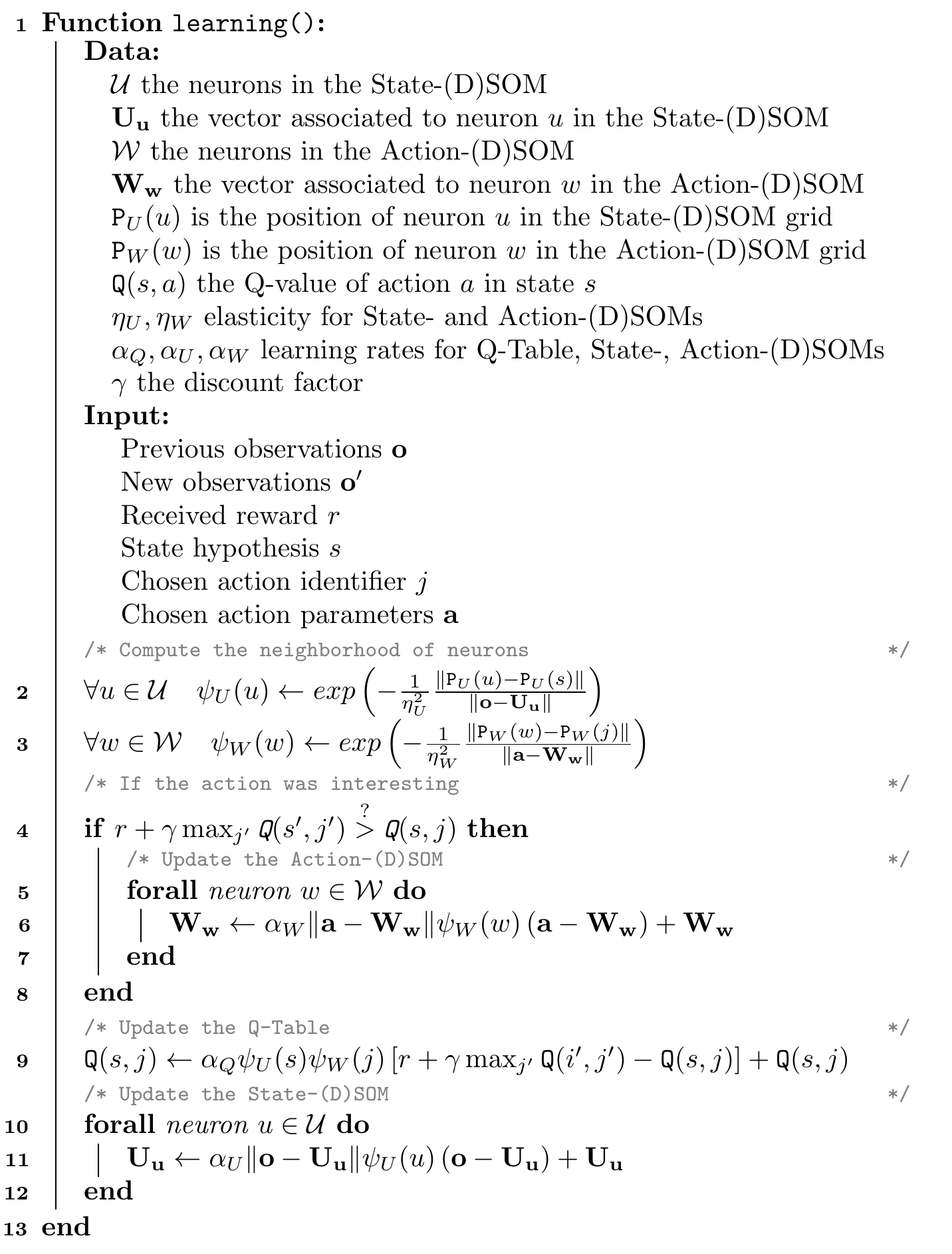
Figure 4.5: Learning algorithm

First, we update the Action-(D)SOM. Remember that we do not have the ground-truth for actions: we do not know which parameters yield the best rewards. Moreover, we explored the action space by randomly noising the proposed action; it is possible that the perturbed action is actually worse than the learned one. In this case, we do not want to update the Action-(D)SOM, as this would worsen the agent’s performances. We thus determine whether the perturbed action is better than the proposed action by comparing the received reward with the memorized interest of the proposed action, using the following equation:

$$\begin{equation} r + \gamma \max_{j'} \Q(s',j') \stackrel{?}{>} \Q(s,j) \tag{4.5} \end{equation}$$

If the perturbed action is deemed better than the proposed one, we update the Action-(D)SOM towards the perturbed action (lines 4-8). To do so, we assume that the Best Matching Unit (BMU), i.e., the center of the neighborhood, is the neuron that was selected at the decision step, $j$ (line 3). We then apply the corresponding update equation, Equation (4.1) for a SOM, or Equation (4.2) for a DSOM, to move the neurons’ prototypes towards the perturbed action.

Secondly, we update the actions’ interests, i.e., the Q-Table (line 9). To do so, we rely on the traditional Bellman’s equation that we presented in the State of the Art: Equation (2.1). However, Smith’s algorithm introduces a difference in this equation to increase the learning speed. Indeed, the State- and Action-(D)SOMs offer additional knowledge about the states and actions: as they are discrete identifiers mapping to continuous vectors in a latent space, we can define a notion of similarity between states (resp. actions) by measuring the distance between the states’ vectors (resp. actions’ vectors). Similar states and actions will most likely have a similar interest, and thus each Q-Value is updated at each time step, instead of only the current state-action pair, by taking into account the neighborhoods of the State- and Action-(D)SOMs (computed on lines 2 and 3). Equation (4.6) shows the resulting formula:

$$\begin{equation} \Q_{t+1}(s,j) \leftarrow \alpha \psi_{U}(s) \psi_{W}(j) \left[r + \gamma \max_{j'} \Q_{t}(s',j') \right] + (1 - \alpha)\Q_{t}(s,j) \tag{4.6} \end{equation}$$

where $s$ was the state hypothesis at step $t$, $j$ was the chosen action identifier, $r$ is the received reward, $s'$ is the state hypothesis at step $t+1$ (from the new observations). $\psi_U(s)$ and $\psi_W(j)$ represent, respectively, the neighborhood of the State- and Action-(D)SOMs, centered on the state $s$ and the chosen action identifier $j$. Intuitively, the equation takes into account the interest of arriving in this new state, based on the maximum interest of actions available in the new state. This means that an action could yield a medium reward by itself, but still be very interesting because it allows to take actions with higher interests. On the contrary, an action with a high reward, but leading to a state with only catastrophic actions would have a low interest.

Finally, we learn the State-SOM, which is a very simple step (lines 10-12). Indeed, we have already mentioned that we know data points, i.e., observations, that have been sampled from the distribution of states by the environment. Therefore, we simply update the neurons’ prototypes towards the received observation at the previous step. Prototype vectors are updated based on both their own distance to the data point, within the latent space, and the distance between their neuron and the best matching unit, within the 2D grid neighborhood (using the neighborhood computed on line 2). This ensures that the State-SOM learns to represent states which appear in the environment.

Remark. In the presented algorithm, the neighborhood and update formulas correspond to a DSOM. When using the Q-SOM algorithm, these formulas must be replaced by their SOM equivalents. The general structure of the algorithm, i.e., the steps and the order in which they are taken, stays the same.

Remark. Compared to Smith’s algorithm, our extensions differ in the following aspects:

• DSOMs can be used in addition to SOMs.
• Hyperparameters are not annealed, i.e., they are constant throughout the simulation, so that agents can continuously learn instead of slowly converging.
• Actions are chosen through a Boltzmann distribution of probabilities based on their interests, instead of using the $\epsilon$-greedy method.
• The random noise to explore the actions’ space is drawn from a Gaussian distribution instead of a uniform one.
• The neighborhood functions of the State- and Action-(D)SOMs is a gaussian instead of a linear one.
• The number of dimensions of the actions’ space in the following experiments is greater (6) than in Smith’s original experiments (2). This particularly prompted the need to explore other ways to randomly noise actions, e.g., the gaussian distribution. Note that some other methods have been tried, such as applying a noise on a single dimension each step, or randomly determining for each dimension whether it should be noised at each step; they are not disclosed in the results as they performed slightly below the gaussian method. Searching for better hyperparameters could yield better results for these methods.

4.5 Experiments

In order to validate our proposed algorithms, we ran some experiments on our Smart Grid use-case that we presented in 3.4.

First, let us apply the algorithms and formal model on this specific use-case. The observation space, $\ObsSpace$, is composed of the information that agents receive: the time (hour), the available energy, their personal battery storage, … The full list of observations was defined in Section 3.4.4. These values range from 0 to 1, and we have 11 such values, thus we define $\ObsSpace_l = [0,1]^{11}$.

Similarly, actions are defined by multiple parameters: consume energy from grid, consume from battery, sell, … These actions were presented in Section 3.4.3. To simplify the learning of actions, we constrain these parameters to the $[0,1]$ range; they are scaled to the true agent’s action range outside the learning and decision processes. For example, let us imagine an agent with an action range of $6,000$, and an action parameter, as outputted by the decision process, of $0.5$, the scaled action parameter will be $0.5 \times 6,000 = 3,000$. We have 6 actions parameters, and thus define $\ActionSpace_l = [0,1]^{6}$.

In the sequel, we present the reward functions that we implemented to test our algorithms, as well as the experiments’ scenarii. Finally, we quickly describe the 2 algorithms that we chose as baselines: DDPG and MADDPG.

4.5.1 Reward functions

We implemented multiple reward functions that each focus on different ethical stakes. Most of them are based on the principle of Difference Reward (Yliniemi & Tumer, 2014b) to facilitate the Credit Assignment, as discussed in Section 2.3.1. Additionally, 2 functions focus on multiple objectives, but with a rather naïve approach (see our next contributions for a better approach), and another 2 focus on adaptation, i.e., the agents’ capacity to adapt their behaviour to changing mores, by making the reward function artificially change at a fixed point in time.

We give an intuitive definition and a mathematical formula for each of these reward functions below.

Equity

Determine the agent’s contribution to the society’s equity, by comparing the current equity with the equity if the agent did not act. The agent’s goal is thus to maximize the society’s equity.

$$\RewardFn_{eq}(agent) = (1 - \texttt{Hoover}(Comforts)) - (1 - \texttt{Hoover}(Comforts \setminus \{agent\}))$$

Over-Consumption

Determine the agent’s contribution to over-consumption, by comparing the current over-consumed amount of energy, with the amount that would have been over-consumed if the agent did not act. The agent’s goal is thus to minimize society’s over-consumption.

$$\RewardFn_{oc}(agent) = 1 - \frac{\mathit{OC}}{\sum_{\forall a} (\mathit{Consumed}_{a} + \mathit{Stored}_{a})} - \frac{\mathit{OC} - (\mathit{Consumed}_{agent} + \mathit{Stored}_{agent})}{\sum_{\forall a \neq agent} (\mathit{Consumed}_{a} + \mathit{Stored}_{a})}$$

Comfort

Simply return the agent’s comfort, so that agents aim to maximize their comfort. This intuitively does not seem like an ethical stake, however it can be linked to Schwartz’ “hedonistic” value, and therefore is an ethical stake, focused on the individual aspect. We will mainly use this reward function in combination with others that focus on the societal aspect, to demonstrate the algorithms’ capacity to learn opposed moral values.

$$\RewardFn_{comfort}(agent) = Comforts_{agent}$$

Multi-Objective Sum

A first and simple reward function that combines multiple objectives, namely limitation of over-consumption and comfort. The goal of agents is thus to both minimize the society’s over-consumption while maximizing their own comfort. This may be a difficult task, because the simulation is designed so that there is a scarcity of energy most of the time, and agents will most likely over-consume if they all try to maximize their comfort. On the contrary, reducing the over-consumption means they need to diminish their comfort. There is thus a trade-off to be achieved between over-consumption and comfort.

$$\RewardFn_{mos}(agent) = 0.8 \times \RewardFn_{oc}(agent) + 0.2 \times \RewardFn_{comfort}(agent)$$

Multi-Objective Product

A second, but also simple, multi-objective reward functions. Instead of using a weighted sum, we multiply the reward together. This function is more punitive than the sum, as a low reward cannot be “compensated”. For example, let us consider a vector of reward components $[0.1, 0.9]$. Using the weighted sum, the result depends on the weights: if the first component has a low coefficient, then the result may actually be high. On contrary, the product will return $0.1 \times 0.9 = 0.09$, i.e., a very low reward. Any low component will penalize the final result.

$$\RewardFn_{mop}(agent) = \RewardFn_{oc}(agent) \times \RewardFn_{comfort}(agent)$$

Adaptability1

A reward function that simulates a change in its definition after 2000 time steps, as if society’s ethical mores had changed. During the first 2000 steps, it behaves similarly as the Over-Consumption reward function, whereas for later steps it returns the mean of Over-Consumption and Equity rewards.

$$\RewardFn_{ada1}(agent) = \begin{cases} \RewardFn_{oc}(agent) & \text{if } t < 2000 \\ \frac{\RewardFn_{oc}(agent) + \RewardFn_{eq}(agent)}{2} & \text{else} \end{cases}$$

Adaptability2

Similar to Adaptability1, this function simulates a change in its definition. We increase the difficulty by making 2 changes, one after 2000 time steps, and another after 6000 time steps, and by considering a combination of 3 rewards after the second change.

$$\RewardFn_{ada2}(agent) = \begin{cases} \RewardFn_{oc}(agent) & \text{if } t < 2000 \\ \frac{\RewardFn_{oc}(agent) + \RewardFn_{eq}(agent)}{2} & \text{else if } t < 6000 \\ \frac{\RewardFn_{oc}(agent) + \RewardFn_{eq}(agent) + \RewardFn_{comfort}(agent)}{3} & \text{else} \end{cases}$$

As we can see, the various reward functions have different aims. Some simple functions, such as equity, overconsumption, or comfort, serve as a baseline and building blocks for other functions. Nevertheless, they may be easy to optimize: for example, by consuming absolutely nothing, the overconsumption function can be satisifed. On the contrary, the comfort function can be satisfied by consuming the maximum amount of energy, such that the comfort is guaranteed to be close to $1$. The 2 multi-objective functions thus try to force agents to learn several stakes at the same time, especially if they are contradictory, such as overconsumption and comfort. The agent thus cannot learn a “trivial” behaviour and must find the optimal behaviour that manages to satisfy both as much as possible. Finally, the adaptability functions go a step further and evaluate agents’ ability to adapt when the considerations change.

4.5.2 Scenarii

In order to improve the richness of our experiments, we designed several scenarii. These scenarii are defined by 2 variables: the agents’ consumption profile, and the environment’s size, i.e., number of agents.

We recall from Section 3.4.6 that learning agents are instantiated with a profile, determining their battery capacity, their action range, and their needs, i.e., the quantity of energy they want to consume at each hour. These needs are extracted from real consumption profiles; we propose 2 different versions, the daily and the annual profiles. In the daily version, needs are averaged over every day of the year, thus yielding a need for each hour of a day: this is illustrated in Figure 4.6. This is a simplified version, averaging the seasonal differences; its advantages are a reduced size, thus decreasing the required computational resources, a simpler learning, and an easier visualization for humans. On the other hand, the annual version is more complete, contains seasonal differences, which improve the environment’s richness and force agents to adapt to important changes.

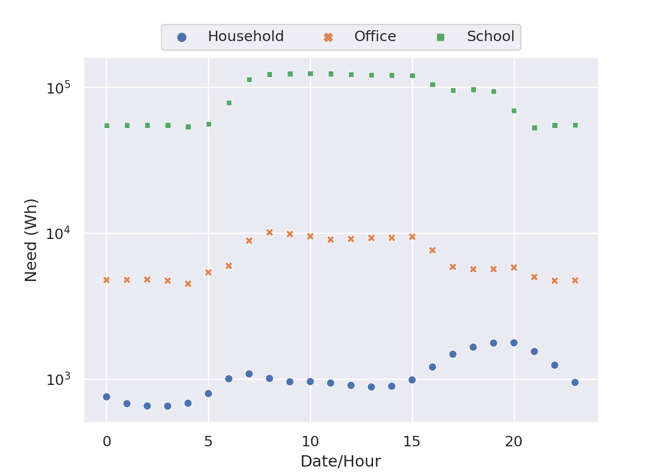
Figure 4.6: The agents’ needs for every hour of the day in the daily profile.

The second property is the environment size. We wanted to test our algorithms with different sets of agents, to ensure the scalability of the approach, in the sense that agents are able to learn a correct behaviour and adapt to many other agents in the same environment. This may be difficult as the number of agents increases, since there will most certainly be more conflicts. We propose a first, small environment, containing $20$ Households agents, $5$ Office agents, and $1$ School agent. The second environment, medium, contains roughly 4 times more agents than in the small case: $80$ Household agents, $19$ Office agents, and $1$ School.

4.5.3 DDPG and MADDPG baselines

In order to prove our algorithms’ advantages, we chose to compare them to the well-known DDPG (Lillicrap et al., 2015) and its multi-agent extension, MADDPG (Lowe et al., 2017).

DDPG, or Deep Deterministic Policy Gradient is one of the algorithms that extended the success of Deep Reinforcement Learning to continuous domains (Lillicrap et al., 2015). It follows the quite popular Actor-Critic architecture, which uses 2 different Neural Networks: one for the Actor, i.e., to decide which action to perform at each time step, and another for the Critic, i.e., to evaluate whether an action is interesting. We chose it as a baseline since it focuses on problems with similar characteristics, e.g., continuous domains, and is a popular baseline in the community.

MADDPG, or Multi-Agent Deep Deterministic Policy Gradient, extends the idea of DDPG to the multi-agent setting (Lowe et al., 2017), by relying on the Centralized Training idea. As we mentioned in Section 2.3.2, it is one of the most used methods to improve multi-agent learning, by sharing data among agents during the learning phase. This helps agents make a model of other agents and adapt to their respective behaviours. However, during execution, sharing data in the same manner is often impracticable or undesirable, as it would impair privacy and require some sort of communication between agents; thus, data is not shared any more at this point (Decentralized Execution). We recall that, as such, Centralized Training - Decentralized Execution makes a distinction between training and execution, and is thus inadequate for continuous learning, and constant adaptation to changes. On the other hand, if we were to make agents continuously learn with centralized data sharing, even in the execution phase, we would impair privacy of users that are represented or impacted by the agents. These reasons are why we chose not to use this setting for our own algorithms Q-SOM and Q-DSOM. While we do not use centralized training, we want to compare them to an algorithm that uses it, such as MADDPG, in order to determine whether there would be a performance gain, and what would be the trade-off between performance and privacy. In MADDPG, the Centralized Training is simply done by using a centralized Critic network, which receives observations, actions, and rewards from all agents, and evaluates all agents’ actions. The Actor networks, however, are still individualized: each agent has its own network, which the other agents cannot access. During the training phase, the Critic network is updated thanks to the globally shared data, whereas Actor networks are updated through local data and the global Critic. Once the learning is done, the networks are frozen: the Critic does not require receiving global data any more, and the Actors do not rely on the Critic any more. Only the decision part, i.e., which action should we do, is kept, by using the trained Actor network as-is.

4.6 Results

Several sets of experiments were performed:

• First, numerous experiments were launched to search for the best hyperparameters of each algorithm, to ensure a fair comparison later. Each set of hyperparameters was run $10$ times to obtain average results, and a better statistical significance. In order to limit the number of runs and thus the computational resources required, we decided to focus on the adaptability2 reward for these experiments. This function is difficult enough so that the algorithms will not reach almost 100% immediately, which would make the hyperparameter search quite useless, and is one of the 2 that interest us the most, along with adaptability1, so it makes sense that our algorithms are optimized for this one. The annual consumption profile was used to increase the richness, but the environment size, i.e., number of agents, was set to small in order to once again reduce the computational power and time.

• Then, the 4 algorithms, configured with their best hyperparameters, were compared on multiple settings: both annual and daily consumption profiles, both small and medium sizes of environment, and all the reward functions. This resulted in $2 \times 2 \times 7$ scenarii, which we ran $10$ times for each of the $4$ algorithms.

In the following results, we define a run’s score as the average of the global rewards per step. The global reward corresponds to the reward, without focusing on a specific agent. For example, the equity reward compares the Hoover index of the whole environment to a hypothetical environment without the agent. The global reward, in this case, is simply the Hoover index of the entire environment. This represents, intuitively, how the society of agents performed, globally. Taking the average is one of the simplest methods to get a single score for a given run, which allows comparing runs easily.

4.6.1 Searching for hyperparameters

Tables 4.1, 4.2, 4.3, 4.4 summarize the best hyperparameters that have been found for each algorithm, based on the average runs’ score obtained when using these parameters.

4.6.2 Comparing algorithms

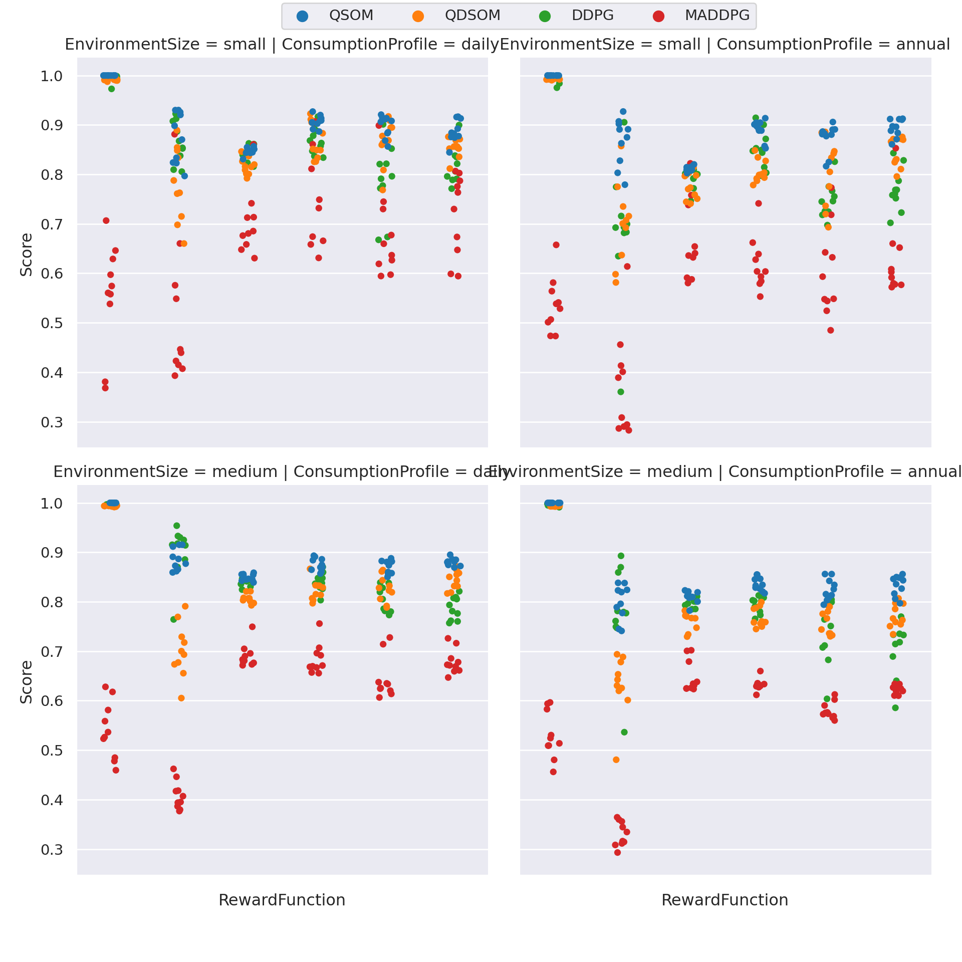
Figure 4.7: Distribution of scores per learning algorithm, on every scenario, for 10 runs with each reward function.

The results presented in Figure 4.7 and Table 4.5 show that the Q-SOM algorithm performs better. We use the Wilcoxon statistical test, which is the non-parametric equivalent of the well-known T-test, to determine whether there is a statistically significant difference in the means of runs’ scores between different algorithms. Wilcoxon’s test, when used with the greater alternative, assumes as a null hypothesis that the 2 algorithms have similar means, or that the observed difference is negligible and only due to chance. The Wilcoxon method returns the p-value, i.e, the likelihood of the null hypothesis being true. When $p < \alpha = 0.05$, we say that it is more likely that the null hypothesis can be refuted, and we assume that the alternative hypothesis is the correct one. The alternative hypothesis, in this case, is that the Q-SOM algorithm obtains better results than its opposing algorithm. We thus compare algorithms 2-by-2, on each reward function and scenario.

The statistics, presented in Table 4.6, prove that the Q-SOM algorithm statistically outperforms other algorithms, in particular DDPG and MADDPG, on most scenarii and reward functions, except a few cases, indicated by the absence of * next to the p-value. For example, DDPG obtains similar scores on the daily / small overconsumption and multiobj-prod cases, as well as daily / medium overconsumption, and annual / medium overconsumption. Q-DSOM is also quite on par with Q-SOM on the daily / small adaptability1 case. Yet, MADDPG is consistently outperformed by Q-SOM.

Figure 4.8 shows the evolution of individual rewards received by agents over the time steps, in the annual / small scenario, using the adaptability2 reward function. We chose to focus on this combination of scenario and reward function as they are, arguably, the most interesting. Daily scenarii are perhaps too easy for the agents as they do not include as many variations as the annual; additionally, small scenarios are easier to visualize and explore, as they contain fewer agents than medium scenarios. Finally, the adaptability2 is retained for the same arguments that made us choose it for the hyperparameters search. We show a moving average of the rewards in order to erase the small and local variations to highlight the larger trend of the rewards’ evolution.

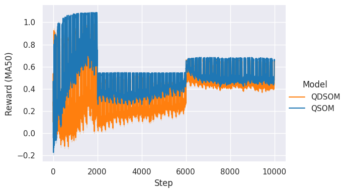
Figure 4.8: Agents’ individual rewards received per time step, over 10 runs in the annual / small scenario, and using the adaptability2 reward function. Rewards are averaged in order to highlight the trend.

We can see from the results that the small scenarii seem to yield a slightly better score than the medium scenarii. Thus, agents are impacted by the increased number of other agents, and have difficulties learning the whole environment dynamics. Still, the results reported for the medium scenarii are near the small results, and very close to $1$. Even though there is indeed an effect of the environment size on the score, this hints towards the scalability of our approach, as the agents managed to learn a “good” behaviour that yields high rewards.

4.7 Discussion

In this chapter, we presented our first contribution consisting in two reinforcement learning algorithms, Q-SOM and Q-DSOM, which aimed to answer the following research question: How to learn behaviours aligned with moral values, using Reinforcement Learning with complex, continuous, and multi-dimensional representations of actions and situations? How to make the multiple learning agents able to adapt their behaviours to changes in the environment?

We recall that the principal important aspects and limitations identified in the State of the Art, and which pertains to our 1st research question, were the following:

• Using continuous and multi-dimensional domains to improve the environment’s richness.
• Continuously learning and adapting to changes in the environment, including in the reward function, i.e., the structure that encodes and captures the ethical considerations that agents should learn to exhibit.
• Learning in a multi-agent setting, by taking into account the difficulties posed by the presence of other agents.

The continuous and multi-dimensional aspect was solved by design, thanks to the SOMs and DSOMs that we use in our algorithms. They learn to handle the complex observations and actions domains, while advantageously offering a discrete representation that can be leveraged with the Q-Table, permitting a modular approach. This modular approach, and the use of Q-Tables, allow for example to compare different actions, which is not always possible in end-to-end Deep Neural Networks. This point in particular will be leveraged in our 3rd contribution, through multi-objective learning, in Chapter 6.

The continuous adaptation was also handled by our design choices, notably by disabling traditional convergence mechanisms. The use of (D)SOMs also help, as the representation may shift over time by moving the neurons. Additionally, our experiments highlight the ability of our algorithms to adapt, especially when compared to other algorithms, through the specific adaptability1 and adaptability2 functions.

Finally, challenges raised by the multi-agent aspect were partially answered by the use of Difference Rewards to create the reward functions. On the other hand, the agents themselves have no specific mechanism that help them learn a behaviour while taking account of the other agents in the shared environment, e.g., contrary to Centralized Training algorithms such as MADDPG. Nevertheless, our algorithms managed to perform better than MADDPG on the proposed scenarii and reward functions, which means that this limitation is not crippling.

In addition to the multi-agent setting, our algorithms still suffer from a few limitations, of which we distinguish 2 categories: limitations that were set aside in order to propose a working 1st step, and which will be answered incrementally in the next contributions; and longer-terms limitations that are still not taken care of at the end of this thesis. We will first briefly present the former, before detailing the latter.

From the objectives we set in this manuscript’s introduction, and the important points identified in the State of the Art, the following were set aside temporarily:

• Interpretable rewards and reward functions constructed from domain expert knowledge: The reward functions we proposed have the traditional form of mathematical formulas; the resulting rewards are difficult to interpret, as the reasoning and rationale are not present in the formula. In this contribution, proposed reward functions were kept simple as a validation tool to evaluate the algorithms’ ability to learn. We tackle this point in the next contribution, in Chapter 5, in which we propose to construct reward functions through symbolic-based judgments.

• Multiple moral values: Some of our reward functions hinted towards the combination of multiple moral values, such as the multi-objective-sum, multi-objective-prod, adaptability1, and adaptability2. However, the implementations of moral values were rather simple and did not include many subtleties, e.g., for the equity, we might accept an agent to consume more than the average, if the agent previously consumed less, and is thus “entitled” to a compensation. We also improve this aspect in the next contribution, by providing multiple judging agents that each focus on a different moral value.

• Multiple moral values / objectives: Moreover, these moral values, which can be seen as different objectives, are simply aggregated in the reward function. On the agents’ side, the reward is a simple scalar, and nothing allows to distinguish the different moral values, nor to recognize dilemmas situations, where multiple values are in conflict and cannot be satisfied at the same time. This is addressed by our 3rd contribution, in Chapter 6, in which we extend the Q-(D)SOM algorithms to a multi-objective setting.

As for the longer-terms limitations and perspectives:

• As we already mentioned, the multi-agent aspect could be improved, for example by adding communication mechanisms between agents. Indeed, by being able to communicate, agents could coordinate their actions so that the joint-action could be even better. Let us assume that an agent, which approximately learned the environment dynamics, believes that there is not much consumption at 3AM, and chooses the strategy of replenishing its battery at this moment, so as to have a minimal impact on the grid. Another agent may, at some point, face an urgent situation that requires it to consume exceptionally at 3AM this day. Without coordination, the 2 agents will both consume an import amount of energy at the same time, thus impacting the grid and potentially over-consuming. On the other hand, if the agents could communicate, the second one may inform other agents of its urgency. The first one would perhaps choose to consume only at 4AM, or they would both negotiate an amount of energy to share, in the end proposing a better joint-action than the uncoordinated sum of their individual actions. However, such communication should be carefully designed in a privacy-respectful manner.

In order to make the reward functions more understandable, in particular by non-AI expert, such as lay users, domain experts, or regulators, to be able to capture expert knowledge, and to allow easier modification, e.g., when the behaviour is not what we expected, we propose to replace the numerical reward functions by separate, symbolic, judging agents. We detail this in the next chapter.

References

Bernstein, D. S., Givan, R., Immerman, N., & Zilberstein, S. (2002). The complexity of decentralized control of markov decision processes. Mathematics of Operations Research, 27(4), 819–840.

Kohonen, T. (1990). The self-organizing map. Proceedings of the IEEE, 78(9), 1464–1480.

Lillicrap, T. P., Hunt, J. J., Pritzel, A., Heess, N., Erez, T., Tassa, Y., … Wierstra, D. (2015). Continuous control with deep reinforcement learning. arXiv Preprint arXiv:1509.02971.

Lowe, R., Wu, Y., Tamar, A., Harb, J., Abbeel, P., & Mordatch, I. (2017). Multi-agent actor-critic for mixed cooperative-competitive environments. Neural Information Processing Systems (NIPS).

Rougier, N., & Boniface, Y. (2011). Dynamic self-organising map. Neurocomputing, 74(11), 1840–1847.

Smith, A. J. (2002a). Applications of the self-organising map to reinforcement learning. Neural Networks, 15(8-9), 1107–1124.

Smith, A. J. (2002b). Dynamic generalisation of continuous action spaces in reinforcement learning: A neurally inspired approach (PhD thesis). University of Edinburgh.

Watkins, C. J., & Dayan, P. (1992). Q-learning. Machine Learning, 8(3), 279–292.

Yliniemi, L., & Tumer, K. (2014b). Multi-objective multiagent credit assignment through difference rewards in reinforcement learning. In Asia-pacific conference on simulated evolution and learning (pp. 407–418). Springer.